CENTRAL TENDENCY
Central tendency (or measure of central tendency) is a central or typical value for a probability distribution ( probability distribution is the mathematical function that gives the probabilities of occurrence of different possible outcomes for an experiment.
More specifically, the probability distribution is a mathematical description of a random phenomenon in terms of the probabilities of events.
For instance, if the random variable X is used to denote the outcome of a coin toss ("the experiment"), then the probability distribution of X would take the value 0.5 for X = heads, and 0.5 for X = tails (assuming the coin is fair). Examples of random phenomena can include the results of an experiment or survey It may also be called a center or location of the distribution ) Colloquially, measures of central tendency are often called averages.
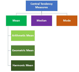
The most common measures of central tendency are the
arithmetic mean,
Median,
Mode
Range
MEAN - The arithmetic mean of a set of observed data is defined as being equal to the sum of the numerical values of each and every observation divided by the total number of observations.
For example, consider the monthly salary of 10 employees of a firm: 2500, 2700, 2400, 2300, 2550, 2650, 2750, 2450, 2600, 2400. The arithmetic mean is
{2500+2700+2400+2300+2550+2650+2750+2450+2600+2400/{10}}=2530.}
If the data set is a statistical population (i.e., consists of every possible observation and not just a subset of them), then the mean of that population is called the population mean. If the data set is a statistical sample (a subset of the population), we call the statistic resulting from this calculation a sample mean.
MEDIAN
In statistics and probability theory, a median is a value separating the higher half from the lower half of a data sample, a population or a probability distribution.
MODE
The mode of a set of data values is the value that appears most often.] If X is a discrete random variable, the mode is the value x (i.e, X = x) at which the probability mass function takes its maximum value. In other words, it is the value that is most likely to be sampled.
Geometric mean is a mean or average, which indicates the central tendency or typical value of a set of numbers by using the product of their values (as opposed to the arithmetic mean which uses their sum). The geometric mean is defined as the nth root of the product of n numbers, i.e., for a set of numbers x1, x2, ..., xn, the geometric mean is defined as
![{\displaystyle \left(\prod _{i=1}^{n}x_{i}\right)^{\frac {1}{n}}={\sqrt[{n}]{x_{1}x_{2}\cdots x_{n}}}}](https://wikimedia.org/api/rest_v1/media/math/render/svg/026cae6801f672b9858d55935ec7397183dc3a36)
For instance, the geometric mean of two numbers, say 2 and 8, is just the square root of their product, that is,

. As another example, the geometric mean of the three numbers 4, 1, and 1/32 is the cube root of their product (1/8), which is 1/2, that is,
![{\displaystyle {\sqrt[{3}]{4\cdot 1\cdot 1/32}}=1/2}](https://wikimedia.org/api/rest_v1/media/math/render/svg/dfd83c4a9ce55b2c53c47b9b32e0e99cf2b92bd8)
.
A geometric mean is often used when comparing different items—finding a single "figure of merit" for these items—when each item has multiple properties that have different numeric ranges.
[For example, the geometric mean can give a meaningful value to compare two companies which are each rated at 0 to 5 for their environmental sustainability, and are rated at 0 to 100 for their financial viability. If an arithmetic mean were used instead of a geometric mean, the financial viability would have greater weight because its numeric range is larger. That is, a small percentage change in the financial rating (e.g. going from 80 to 90) makes a much larger difference in the arithmetic mean than a large percentage change in environmental sustainability (e.g. going from 2 to 5). The use of a geometric mean normalizes the differently-ranged values, meaning a given percentage change in any of the properties has the same effect on the geometric mean. So, a 20% change in environmental sustainability from 4 to 4.8 has the same effect on the geometric mean as a 20% change in financial viability from 60 to 72.
The geometric mean can be understood in terms of geometry. The geometric mean of two numbers,

and

, is the length of one side of a square whose area is equal to the area of a rectangle with sides of lengths
and
. Similarly, the geometric mean of three numbers,
,
, and

, is the length of one edge of a cube whose volume is the same as that of a cuboid with sides whose lengths are equal to the three given numbers.
The geometric mean applies only to positive numbers. It is also often used for a set of numbers whose values are meant to be multiplied together or are exponential in nature, such as data on the growth of the human population or interest rates of a financial investment.
The geometric mean is also one of the three classical Pythagorean means, together with the aforementioned arithmetic mean and the harmonic mean. For all positive data sets containing at least one pair of unequal values, the harmonic mean is always the least of the three means, while the arithmetic mean is always the greatest of the three and the geometric mean is always in between.
Harmonic mean
H of the positive real numbers

is defined to be

The third formula in the above equation expresses the harmonic mean as the reciprocal of the arithmetic mean of the reciprocals.
From the following formula:

it is more apparent that the harmonic mean is related to the arithmetic and geometric means. It is the reciprocal dual of the arithmetic mean for positive inputs:

The harmonic mean is a Schur-concave function, and dominated by the minimum of its arguments, in the sense that for any positive set of arguments,

. Thus, the harmonic mean cannot be made arbitrarily large by changing some values to bigger ones (while having at least one value unchanged).
weighted arithmetic mean
Is similar to an ordinary arithmetic mean (the most common type of average), except that instead of each of the data points contributing equally to the final average, some data points contribute more than others. The notion of weighted mean plays a role in descriptive statistics and also occurs in a more general form in several other areas of mathematics.
If all the weights are equal, then the weighted mean is the same as the arithmetic mean. While weighted means generally behave in a similar fashion to arithmetic means, they do have a few counterintuitive properties, as captured for instance in Simpson's paradox.
Example
it
Given two school classes, one with 20 students, and one with 30 students, the grades in each class on a test were:
- Morning class = 62, 67, 71, 74, 76, 77, 78, 79, 79, 80, 80, 81, 81, 82, 83, 84, 86, 89, 93, 98
- Afternoon class = 81, 82, 83, 84, 85, 86, 87, 87, 88, 88, 89, 89, 89, 90, 90, 90, 90, 91, 91, 91, 92, 92, 93, 93, 94, 95, 96, 97, 98, 99
The mean for the morning class is 80 and the mean of the afternoon class is 90. The unweighted mean of the 80 and 90 is 85, so the unweighted mean of the two means is 85. However, this does not account for the difference in number of students in each class (20 versus 30); hence the value of 85 does not reflect the average student grade (independent of class). The average student grade can be obtained by averaging all the grades, without regard to classes (add all the grades up and divide by the total number of students):

Or, this can be accomplished by weighting the class means by the number of students in each class. The larger class is given more "weight":

Thus, the weighted mean makes it possible to find the mean average student grade without knowing each student's score. Only the class means and the number of students in each class are needed.
Convex combination exampleEdit
Since only the relative weights are relevant, any weighted mean can be expressed using coefficients that sum to one. Such a linear combination is called a convex combination.
Using the previous example, we would get the following weights:


Then, apply the weights like this:

Mathematical definition
EditFormally, the weighted mean of a non-empty finite multiset of data

with corresponding non-negative weights

is

which expands to:

Therefore, data elements with a high weight contribute more to the weighted mean than do elements with a low weight. The weights cannot be negative. Some may be zero, but not all of them (since division by zero is not allowed).
The formulas are simplified when the weights are normalized such that they sum up to

, i.e.:
 .
.
For such normalized weights the weighted mean is then:
 .
.
Note that one can always normalize the weights by making the following transformation on the original weights:
 .
.
Using the normalized weight yields the same results as when using the original weights:

The ordinam9ry mean

is a special case of the weighted mean where all data have equal weights,

.
The
standard error of the weighted mean (unit input variances),

can be shown via uncertainty propagation to be:

- Truncated mean or trimmed mean
- is a statistical measure of central tendency, much like the mean and median. It involves the calculation of the mean after discarding given parts of a probability distribution or sample at the high and low end, and typically discarding an equal amount of both. This number of points to be discarded is usually given as a percentage of the total number of points, but may also be given as a fixed number of points.


You have shared a lot of information in this article. I would like to express my gratitude to everyone who contributed to this useful article. Keep posting. Tax Accounting Firm In Calgary
ReplyDelete